Plotting Geo data

Data input and processing

This one was a fun one. During my project i had a list of samples we used, and each sample had some minor geopgraphical data attatched from where we got it. Unfortunately we didn’t have a lot of details on some of them (like town, or coordinates) so to keep it comparable we sticked to province level.

I personally don’t like tables, i’m a visual person and a map with dots works way easier for me than a list with province names (half of which i probably never even seen before, and would need a map to even figure out where they are). So let’s get started.

First of, we decided to use shapefiles as our basis to draw maps, we don’t like to make our maps by hand. We obtained these maps from geographical database sites. Next we had two countries in which we had samples, New Zealand and France. On this basis i wrote this script

The script starts out by adding two function to just about ALL my scripts. Both were stolen from StackOverflow, with some minor tweaks here and there maybe. Unfortunately i can’t find the original poster anymore and i truly regret not storing their info.

This first function essentially removes all loaded packages, this is really handy when packages are used that conflict, in my case i often use plyr and dplyr together… they don’t gell well together as they are different forks of the same thing.

DetachAllPackages <- function() {
  basic.packages <- c("package:stats","package:graphics","package:grDevices","package:utils","package:datasets","package:methods","package:base")
  package.list <- search()[ifelse(unlist(gregexpr("package:",search()))==1,TRUE,FALSE)]
  package.list <- setdiff(package.list,basic.packages)
  if (length(package.list)>0)  for (package in package.list) detach(package, character.only=TRUE)
}

Now we can use the followin line to detach all packages

DetachAllPackages()

Next function is an easy package evaluator. It will check if the packages is already installed, and if not it will install it first. If the packages is installed, it will evaluated if it’s already loaded and if not it will load it. This saves a lot of waiting and prevents installing stuff over and over.

install_load <- function(Required_Packages) {
  for(package in Required_Packages){
    if (!package %in% installed.packages()) install.packages(package, character.only = TRUE)
    library(package, character.only = TRUE)
  }
}

And packages can now simply be loaded by

install_load(c("your_package","your_second_package","etc"))

For my example my data is an excell sheet with different samples with different columns of locational data, and i found tmap the best looking approach to make maps in R. So we’ll be using those for this example.

We’ll start with the openxlsx package to open the excell file, plyr package for the “count” function.

install_load(c("openxlsx","plyr"))

So now that those are installed and loaded, we’ll open our data.

table_input <- read.xlsx("Sequenced_samples.xlsx", colNames = TRUE,
                         rowNames = FALSE, na.strings=c("","NA"))

Which looks as followed

##   Strain.ID          Town  District     Region     Country
## 1         1 Arthur's Pass    Selwyn Canterbury New Zealand
## 2         4       Te Anau Southland  Southland New Zealand
## 3       142         Tihoi     Taupo    Waikato New Zealand
## 4       142         Tihoi     Taupo    Waikato New Zealand

For this example i wanted to summarize the number of samples per provice, and did this by summarizing all samples for a region. But you could leave this out and just plot all the inidividual regions or towns they are from.

sumSamples <- count(table_input, var=c("Region", "Country")) 
sumSamples$Region <- lapply(sumSamples$Region, function(x) paste(x, " Region"))

We just used plyr, but we need dplyr for the next step so we’ll detach all packages and load our next list.

DetachAllPackages()
install_load(c("ggplot2","colorspace","tmaptools","dplyr","maps","tmap","sf","sp"))

Now we have to load our shapefile… you can get these from all sorts of sources. Sometimes is a census bureau or government website… the shapefiles can also contain different sorts of data so make sure you get what you are looking for. In my case i searched for shapefiles of regional counsils of New Zealand (provinces).

#Get geo data for regional counsils
nzgeo_file <- "nzgeo/REGC2017_GV_Clipped.shp"
#Check if the files actually exists, although this is not really functional, more for my debugging purposes
if (file.exists(nzgeo_file)){
  print("File accepted")
  nzgeo <- read_shape(file=nzgeo_file, as.sf = TRUE)
}

## [1] "File accepted"

Once loaded, i wanted to add the sample sizes per region in the exact centre of the region, so i used the st_centroid function to calculate all the centroids of each province shape.

Then i did the same for France.

frgeo_file <- "frgeo/regions-20170102.shp"
if (file.exists(frgeo_file)){
  print("File accepted")
  frgeo <- read_shape(file=frgeo_file, as.sf = TRUE)
}

print("File accepted")

## [1] "File accepted"

And removed some regions that were too small or islands in the pacific by looking at the shapefile summary, determine the lines that had regions i wanted to ommit, and just removed them based on a matching value in a colum, in this case the insee colum (this column name is off course shapefile depedant)

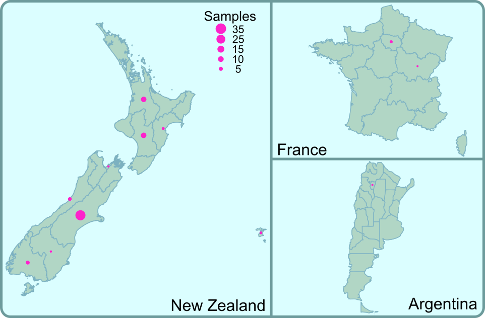
I cheated the system a bit by not merging my summary table with the shapefile… but instead just manually added the values. It could be done automatically but it would have taken more time, and result would have been the same.

nzgeo_centroids$Samples <- c(0,0,10,0,0,3,0,10,0,5,33,2,5,0,2,0,3)
frgeo_centroids$Samples <- c(0,0,0,0,0,0,1,0,0,2,0,0,0)

And now there is nothing left but plotting the maps of the two countries. First New Zealand, which we stored in the variable newzealand_shape_plot. Which looks something like this

newzealand_shape_plot <- tm_shape(nzgeo) +
  tm_layout(bg.color="#f4f3ff", 
            frame="#d9d1ff", 
            frame.lwd=3, 
            main.title="Sample distribution",
            asp = 2) +
  tm_fill("#b2d8c5") +
  tm_borders(col = "#0c94a7",  #Province borders around the provinces
             lwd = 1, 
             lty = "solid", 
             alpha = 0.4)+
  tm_shape(nzgeo_centroids) + #These are the positions of the datapoints
  tm_symbols(col = "#d726f1",  #These are the types of symbol used on the position
             size = "Samples",
             scale = 1.4,
             title.size="Samples per region",
             border.lwd=NA)

Followed by the France plot, which we stored in france_shape_plot.

france_shape_plot  <-   tm_shape(frgeo2) +
  tm_layout(bg.color="#f4f3ff", 
            frame="#d9d1ff", 
            frame.lwd=3,
            asp = 1) +
  tm_fill("#b2d8c5") +
  tm_borders(col = "#0c94a7", #Province borders around the provinces
             lwd = 1, 
             lty = "solid", 
             alpha = 0.4)+
  tm_shape(frgeo_centroids) + #These are the positions of the datapoints
  tm_symbols(col = "#d726f1",  #These are the types of symbol used on the position
             size = "Samples",
             scale = 0.6,
             legend.size.show = FALSE,
             border.lwd=NA) 

Because we stored the two plot in variables we can now plot them in a side by side window. Unfortunately it seems that the tmap packages isn’t as lenient in multi frame plots, it still does a decent job. And CorelDraw, Adobe Illustrator, even InkScape or any other vector based graphical software can be used to correct some orientation issues, as long as you save the final plot as a PDF.

tmap_arrange(newzealand_shape_plot, france_shape_plot, nrow=1,ncol=2)